Department of Physics
Mercer University
Macon, Georgia
June 2005
With the right choice of sensor, a `simple' pendulum has great potential as a seismometer with superior low frequency sensitivity.
Functionality of a seismometer depends on the inertial properties of its `mass'. To measure vertical motions of the earth, the simplest `instrument' is a mass suspended at the end of a spring. Horizontal motions may be detected by a simple pendulum. Complete determination of acceleration at a point on the surface of the earth requires three independent units; i.e., (i) one vertical sensor, and (ii) a pair of horizontal sensors placed in quadrature, such as one operating east /west and the other north/south. (Alternatively, the output from three sensors can be combined to yield the same result, by placing them in a homogeneous triaxial arrangement, as in the Streckeisen STS-2.)
One of the earliest forms of seismometer was simply a mass suspended by an `inextensible' string. In the absence of acceleration, the string orients along the direction of the local vertical; i.e., a plumb bob. If the ground accelerates horizontally at a constant a, along a direction to which the pendulum responds, then the steady-state deflection of the pendulum is opposite the direction of a and of magnitude
|
(1) |
The simplicity of this response is one of the greatest attributes of the conventional pendulum.
The simple pendulum lost favor because it has no means for `mechanical magnification'; therefore, it was replaced by instruments having greater (at higher frequencies) sensitivity.
A common form of horizontal seismometer, frequently referred to as a `pendulum' is a swinging `door' or `garden-gate'. As the axis of the gate approaches the direction of local g, the potential energy function becomes more shallow. The weakening of the restoring torque results in a longer period of the motion for an instrument excecuting simple harmonic oscillation (free-decay following an impulsive disturbance). If all the materials of the gate were `perfect' (obeying Hooke's law) then the sensitivity of this form of accelerometer could become truly great as the axis approaches vertical. Instead of eq.(1), the ideal response of this instrument to a constant acceleration (after all transients have died) is given by
|
(2) |
involving a multiplicative factor (mechanical magnification = 1/sina), where a is the angle the axis makes with respect to the vertical.
The mechanical response of a real-world garden-gate pendulum does not obey eq.(2) as a ® 0, because of the anelastic materials of which the pendulum is constructed. As the period is lengthened by reducing a toward zero, creep processes become ever more significant[1]. Such response afflictions due to anelasticity also make their presence known in vertical instruments designed to operate at long periods. The first truly successful method employed to increase mechanical responsivity of a vertical instrument was the LaCoste zero-length spring. More recent instruments using force-balance by means of a feedback network employ astatic springs that serve a similar purpose. All seismic instruments that use mechanical magnification, depart from ideal behavior at low frequencies; and their performance is limited because of mesoanelastic complexity.
The problem with mechanical magnification is that it not only magnifies the ideal response of the instrument, but it also magnifies the myriad imperfections that manifest themselves at low energies of oscillation. The energy of a mechanical oscillator is given by
|
(3) |
where w = 2p/T is the angular frequency and A is the amplitude of harmonic oscillation. The energy is proportional to both the square of the frequency and the square of the amplitude. As either gets small, or as in the cases of increasing interest to geoscience; when both get small, mesoscale quantization of defect structures invalidates the classical mechanics from which various equations are derived, such as eq(2)[2]. The metastabilities and hysteresis that characterize this regime are important not only to seismometry, but also other fields of research, such as the laser interferometer gravitational observatory (LIGO)[3].
Mechanical oscillators rarely free-decay according to a linear damping model, following an impulsive disturbance. If the damping were due to air surrounding the seismic mass, then the linear model would be a much better approximation. Actual oscillators dissipate energy in the spring through (i) heat, and (ii) structural rearrangements. Classical heat loss (thermoelastic damping) is important at high frequencies, whereas structural rearrangements are important at low frequencies[4]. Structural rearrangement damping is fundamentally nonlinear, and it invalidates, at low frequencies, the use of commonly employed tools for the estimatation of seismometer noise. For example, the noise floor of seismometers is commonly calculated on the basis of the equipartition theorem; i.e., a brownian noise estimate. Formally, such a calculation proceeds as follows [5] (see p. 84): ``for every square term in the Hamiltonian there is 1/2 kT of thermal energy'', where T is the absolute (Kelvin) temperature, and k is the Boltzmann constant.
The problem with seismometer springs is that there is never a single pair of terms (one potential, the other kinetic) in the Hamiltonian, associated with the excitation of a Hooke's law (idealized) spring. There are a large number of quadratic terms in the potential function, the number of which cannot be presently estimated from first principles [6]. Such complexities are also a reason low mass instruments of micro-electromechanical-systems (MEMS) type do not function as had been simplistically theorized. When dealing with small masses, the transition from damping of continuum type to discrete type becomes more important. In larger systems, the number of ways in which `hysteron' energy packets of the order of 10-11J may be distributed is much greater. The `averaging' that results from this large-number statistics is cause for a smooth (gaussian) distribution. Such is not the case for small systems operating at small energies.
Instead of being a parabola, the potential function of a seismometer is complex, containing (local) metastabilities as a type of fine structure superposed on the parabola. The resulting `raggedness' is not quantized at the atomic scale, but rather at the mesoscale (consistent with grain sizes of polycrystalline metallic materials of which seismic springs are fabricated). The potential function is not even stationary, as pictured in the top graph of figure 1; which is commonly employed to explain damping. Rather, the damping mechanism functions more like the illustration of the bottom graph of figure 1.
With the goal of improving low-frequency seismometer performance, it is clear that a tradeoff exists between mechanical magnification and electronics `magnification' (sensor/amplifier gain). Mechanical magnification is limited (in the absence of force-feedback) by the very creep processes that disallow the instrument from performing well at low frequencies. The maximum magnification consistent with long-term stabiity, is very useful for high frequency seismic observations. It is the very reason long-period vertical LaCoste spring instruments worked so well in the WWSSN for detecting earthquake body-waves. Because they operated with a Faraday law (velocity) sensor, there was no means for assessing their performance at mHz frequencies. With the advent of force-balance instruments, great interest has developed in the study of the Earth's eigenmodes (persistent hum). At these low frequencies it is now known that the mechanical magnification that was so useful at higher frequencies-can be detrimental.
The simple pendulum, consistent with eq(1) has zero mechanical magnification. It is an obvious `benchmark' with which to conduct tradeoff studies concerned with the relative merits of mechanical enhancement versus electronic enhancement. In the early days of seismometry, the pendulum quickly lost favor to instruments having mechanical magnification; since in those days there were no good sensors of the motion. Since electronic sensing has improved dramatically in the last twenty years, it is time to reconsider the conventional pendulum. The present experiments show that it is much more useful than simply as a pedagogical tool with which to compare other instruments.
Presently, the most successful, inexpensive sensors of inertial mass movement are (i) optical, and (ii) capacitive. Both are essentially noninvasive, and capacitive devices are the more common. Whether the increasing use of interferometers involving a laser should eventually take preeminence remains to be seen.
There are two ways that parallel plate electrodes of a capacitive sensor may be configured to operate, either in terms of (i) gap-space -variation, or (ii) area-variation. All commercial instruments known to this author operate on the basis of gap-variation. In the force-balance instruments the spacing between electrodes is maintained smaller than 1 mm, with an area of each electrode being several cm2. For a pendulum, it is not the preferred embodiment of capacitive sensor. The natural embodiment for most seismic sensing at low-frequencies is one based on area-variation.
The tutorial of figure 2 describes the operation of a single-element symmetric differential capacitive (SDC) sensor[7]. It is a variant of the first-to-be-discovered technology that is finding its way into MEMS and other devices. It is an example of what has come be known as `fully differential' (now used to describe operational amplifiers as well as sensors).
A key to understanding this device is to recognize that charge cannot be induced through a grounded plate; i.e., a Faraday shield. Thus, in figure 2, the capacitance between any pair of adjacent static electrode elements depends on the amount of area common to the pair; i.e., is not `shadowed' by some portion of the grounded moving electrode. With the moving electrode centered (left case), the bridge is balanced, yielding no output voltage from the amplifier. With the moving electrode at its left-maximum displacement (center case), the a to e and b to d capacitances have been reduced to zero (ignoring fringe fields). Simultaneously, the a to c and b to f capacitances have increased to their maximum value. This unbalancing of the bridge results in a polarity of the output voltage (by means of the diodes) that is opposite to that of the case with the moving electrode positioned at its right-maximum displacement (right case).
Because the capacitance is proportional to the area (itself proportional to the displacement), the sensor is very linear as compared to other capacitive devices. Fringe fields typically cause a small deviation from linear that is cubic in the residuals.
The sensor electronics of the present experiment does not use diodes as shown in the figure 2 tutorial. Rather, the d.c. output is generated using synchronous detection. This yields better stability and signal to noise ratio.
Illustrated in figure 3 is the sensor array used in the instrument of the present study. By connecting four single-element SDC sensors in electrical parallel, the sensitivity is increased by an approximate factor of four. Whereas the electrodes are rectangular in figure 2 (for measuring translation), those of figure 3 are tailored for rotation. For the indicated radii, the following relation insures that all segments have the same area and thus contribute equally to the output:
|
(4) |
Note: The moving electrode set in figure 3 shows an extended section of copper used for damping by means of eddy currents (by placing powerful rare-earth magnets in-front-of and behind the section). The present experiment did not use any external damping means.
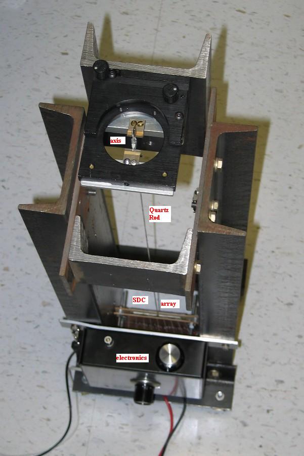
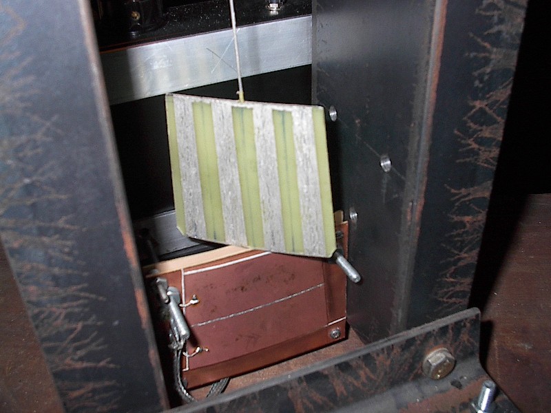
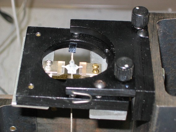
Pictured in figure 4 is a top view of the instrument, and figure 5 is a photograph of the sensor array. To see the moving electrodes, which also serve as the `bob' of the pendulum; the pendulum was lifted from its operational position.
To minimize axis friction, a pair of diamond points were taken from phonograph styluses. These were epoxied in an aluminum yoke, as was the 2 mm dia fuzed quartz rod, that passes all the way through the yoke by way of a center-drilled hole. Glued on the top end of the rod is a small front-surface mirror (piece from a polished silicon wafer), that is used with a He-Ne laser to calibrate the instrument. By means of this optical lever, the calibration constant of the pendulum was measured (for the highest-gain setting of the electronics) to be 5800 V/radian.
The pair of sapphire plates, on which the diamond points rest, are mounted to an adjustable platform (excessed optical mirror mount). By means of the two knurled screws, visible in figure 6, the pitch and roll angles of the platform are adjusted so that (i) the moving electrodes are centered between the opposing set of stationary plates, and (ii) the quartz rod hangs vertically without bending. Adjustments of pitch and roll are made after the housing of the instrument is made plumb by means of bubble levels.
To demonstrate the performance of this conventional pendulum instrument, recorded data from four earthquakes is provided. Two of these were the large Indonesian earthquakes of (i) 26 December 2004, and (ii) 28 March 2005. Their magnitudes were 9.2 and 8.7 respectively. Shown in figure 7 are compressed-time records of each.
The records differ significantly in terms of first response to body waves. Perhaps this is consistent with the fact that the first earthquake caused a devastating tsunami, whereas the second one did not. Because the pendulum is not externally damped, and because the first disturbances are in frequency close to the resonance frequency of the pendulum at 0.7 Hz, there is a great deal of transient motion in the early part of both records. If the instrument were to be used for body-wave studies, these transients could be removed by adding the eddy-current damping subsystem discussed earlier.
The later arriving surface waves are at low-enough frequency that the recorded waveforms are for them a good representation of the earth's acceleration. Examples are provided in figure 8.
Additionally in each of the figure 8 graphs, a short piece of the early record has been expanded in time to resolve the high frequency motions caused by the body waves.
Shown in figure 9 is a 2048 point FFT computed 50 minutes after the start of the 26 Dec earthquake. The surface waves are at their lowest frequency of 17.6 mHz at this time, with a signal level of 57 mV. Using the calibration constant of 5800 V/rad, the pendulum displacement was estimated to be 9.8 mrad. This corresponds to an acceleration of 96.mm/s2, or a ground displacement amplitude of nearly 8. mm.
It should be noted that the ordinate scale of the time plot in figure 10 corresponds to a total range of 0.5 V, whereas that in figure 9 is four times larger at 2.0 V.
Both of the large Indonesian earthquakes had free-earth oscillations associated with them. Examples are provided in figures 11 and 12.
Shown in figure 13 are records for the earthquakes: (i) in Chile, 13 June 2005 and (ii) off the coast of northern California, 15 June 2005. As seen from figures 14 and 15, the lowest observed frequencies were higher for this pair than those derived from the Indonesian earthquakes. The delay of their occurrence, relative to start of the body waves, were significantly shorter. This is consistent with the greater dispersion caused by the long oceanic path in the case of the Indonesian earthquakes.