Soup-can Pendulum

Copyright 2000 by Randall D. Peters

Department of Physics
1400 Coleman Ave.
Mercer University
Macon, Georgia 31207

Abstract

In these studies, a vegetable can containing fluid was swung as a pendulum by supporting its end-lips with a pair of knife edges. The motion was measured with a capacitive sensor and the logarithmic decrement in free decay was estimated from computer collected records. Measurements performed with nine different homogeneous liquids, distributed through six decades in the viscosity h, showed that the damping of the system is dominated by h rather than external forces from air or the knife edges. The log decrement was found to be maximum (0.28) in the vicinity of h = 0.7 Pa·s and fell off more than 15 fold (below 2 ×10^-2) for both small viscosity (h < 1×10^-3 Pa·s) and also for large viscosity (h > 1 ×10³ Pa·s). A simple model has been formulated, which yields reasonable agreement between theory and experiment by approximating the relative rotation of can and liquid.

1  Introduction

Pendulum damping is usually thought of as originating from forces external to the oscillating member-as for example, from air or knife edges. There are many mechanical oscillators, however, for which the primary damping mechanism is internal friction. A recently studied example is that of the long-period pendulum [1]. The present paper describes another pendulum, whose period is short ( <  0.5 s), and which is also influenced primarily by internal friction. The study was partly motivated by the mechanics of rolling vegetable cans. Although a proper interpretation of some results can be tricky[2], it has become commonplace for physics teachers and their students to compare the rolling speed of two different vegetables on an inclined plane. The popularity of these demonstrations suggested that it might also be fascinating to study a ``pendulating" vegetable can. Part of the fascination with the soup-can pendulum derives from early observations in which behavior differences of the type illustrated in Fig. 1 were noted.

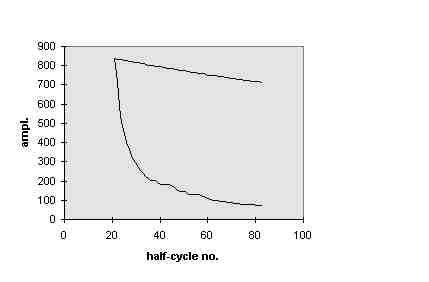
Figure 1. Comparison of the decay of two different vegetable cans.

Shown in this figure is the decay in peak-to-peak amplitude of the motion for each of two different vegetables: (i) blackeyed peas, and (ii) sweet peas. Unlike the blackeyed peas case, for which there is little damping, a dramatic loss occurs when the pendulum is a can of sweet peas. The vertical axis of this graph is peak-to- peak amplitude of the pendulum motion based on analog to digital counts (described later), and it is plotted versus time expressed in half-cycle integers. In all studies presently reported, the period of oscillation is in the vicinity of 0.45 s, using common vegetable cans of size 7.4 cm dia. by 11.2 cm length, and 56 g empty can mass. Although some variations in period were noted from case to case, as expected; these changes were small compared to the primary variation, which is the damping. Later studies are planned in which the second order effects of period will be addressed. The remarkable difference between the sweet peas and blackeyed peas was not anticipated by means of other comparisons. For example, shaking the cans revealed a significant volume of water packed with each of the vegetables. In a rolling comparison it was found that the sweet peas were faster than the blackeyed peas down an incline, but not with a huge difference as in Fig. 1. Another interesting feature of Fig. 1 are the ``steps" in the decay of the sweet peas. Apparently the peas tend to organize in groups, the size of which depends on pendulum amplitude. Thus there is evidence for granularity giving rise to self-organized criticality[3]. The understanding of these effects must also await future studies.

2  Pendulum Design

Shown in Fig. 2 are (i) the support structure for the pendulating can and (ii) the placement of the symmetric differential capacitive (SDC) sensor to monitor position.


Figure 2. Illustration of the soup-can pendulum.

The fixed electrodes of the sensor were attached to the support frame with super glue, near the top end of the can, using two pieces of 8 mm thick lucite. The frame was constructed from a 11 cm long section of ``c" channel aluminum of 8 mm wall thickness and 15.3 cm width. Two small aluminum pieces to hold the knife edges were welded to the 4 cm high sides, using a tungsten inert gas, or TIG welder. These optionally could have been attached with screws. The clearance between the bottom of a can and the frame is » 1 cm. The knife edges were made from a section of bandsaw blade 0.5 mm thickness, 1.2 cm width. The teeth were ground off the blade, and each knife edge was sharpened in the vicinity of the end which contacts the lip of the can. One of these was press fitted into a slot cut in its small aluminum holder, and the other was hinged with a small steel pin so that the can may be easily mounted and dismounted from the frame. The doubly differential capacitive sensor, which is described elsewhere [4] comprises two sets of stationary electrodes held in parallel proximity, and a third planar electrode which moves between the stationary pair. For the present experiments, the moving electrode was cut with scissors from thin sheet aluminum. A near right angle bend in the lower section of this ``fan-shaped" piece permits it to be fixed in position on top of the can by a small magnet.

3  Experimental Technique

When filled with inhomogeneous vegetables, the motion of the can pendulum is hopelessly complicated, relative to a first effort at theoretical modelling of the system. The difficulty of such a task may be appreciated by simply inspecting the sweet pea decay case of Fig. 1. For this reason we chose to first look at decays (for serious study) in which the can is filled with a variety of different homogeneous liquids, whose primary difference is their viscosity, h. In the results which follow, it will be seen that a range in h of more than six orders of magnitude is readily achieved, using only liquids which are common to most physics departments. To insure a meaningful comparison among runs with different liquids, the vegetable can selected for use was in all cases the one whose dimensions were indicated in the discussion of Fig. 1. Following the purchase of a can from the grocery store, the vegetable contents had to be emptied. To facilitate mechanical integrity after refilling, the lid was separated from the body of the can using a can-opener (Culinare) that cuts through the narrow outside crimp in the end-lip. Not only does this technique result in safe products of separation, since there are no sharp edges on either the can or its lid; but also their smooth separation permits the pair to be rejoined, after filling with a test liquid, by means of a thin layer of glue.

3.1  Data Collection

The analog data from the sensor electronics is input to the 33 MHz 486 PC computer by means of a Metrabyte 1401 analog to digital (A/D) converter. Software of both acquisition and processing types was written in QuickBasic (compiled), and the hybrid code had in some cases been written by Metrabyte and in other cases by the author. Two different modes of operation are employed. The setup mode is a real-time one in which the duration of the record graphed on the monitor, and the full-scale sensitivity of the electronics, are chosen after a prompt is displayed. This permits the operator to adjust the electronics offset for a mean output that is in the vicinity of zero. The pendulum displacement is mapped vs time on the monitor using the 'pset' software command. In this mode, the computer emulates an old-fashioned strip-chart recorder. The second mode is one in which a record of 2048 points (2 K) is written to memory of the computer for later analysis. During collection of the record, no graphical information is available for viewing. For all cases presently reported, the 2 K records from which figures were produced, were collected using a full scale sensitivity of (+/-) 0.1 V. For the sensor used in these experiments, the calibration constant corresponding to this A/D sensitivity, was 1.5 ×10⁵ counts/rad for counts in the range -4095 to 4096.

It is possible to view the raw data directly, as illustrated in Fig. 3, which shows the vast difference between a can filled with glycerin and a reference case for which there is insignificant internal friction.

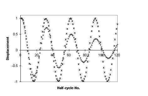
Figure 3 Decay of glycerin compared to a reference decay.

For this comparison, the ordinate values were normalized to the initial peak amplitude, which is a straightforward operation with the Microsoft Excel software that was used to produce all graphs. For a given case, one simply imports from memory to Excel the 2 K record of interest, and then responds to prompts generated by the chart ``wizard". The abscissa values (time) are integer ·Dt where Dt = 30 s/2048. In addition to the obvious difference between the decay constants in the two cases of Fig. 3, one can also see that the period of the motion is slightly greater when the can contains glycerin. As compared to the huge difference in damping coefficients, the variation with period is second order, as previously mentioned. To produce the reference decay, brass weights were fixed inside an empty can (56 g mass), the amount selected to approximate the mass of a water filled can (510 g). The log decrement in this reference (5.0 (+/-) 0.4×10^-3, R²  =  0.993) is evidently influenced largely by the knife edges. By contrast, the empty can (8.1 (+/-)  0.9×10^-3, R²  =  0.998) is evidently influenced primarily by the viscosity of surrounding air.

The decay constant which is referred to as the log decrement is defined as

where q_N and q_N+1 are the displacements of a pair of turning points of like sign separated in time by one period of the oscillation.

In a graph which follows (Fig. 6) of pendulum damping versus viscosity, the reference damping was subtracted from the measured damping to yield the internal friction part. Only at low values of the damping was this correction significant.

4  Theoretical Model

The system was modelled by two coupled differential equations:

where q is the angular displacement of the can, and q_L is associated with the liquid in an ``effective" sense. The constant c is the one adjustable parameter in the model, and h is the viscosity. Being concerned primarily with trends in the damping versus viscosity, the term that would normally multiply the term in q has been set to unity. Thus the period of oscillation of the model system is 6.28 when h  =  0, rather than the actual experimental period in the neighborhood of 0.45 s.

The model equations were first tested in a limiting simple case; i.e., by removing the q term in Eq. (2) and noting that [(q)\dot] and [(q_L)\dot] approach a common value exponentially, with a time constant inversely proportional to h^1/2. To solve (2) and (3) numerically, they were first rewritten as an equivalent coupled set of four first order equations:

Although the liquid motion is undoubtedly complicated in most cases, a simplifying assumption has been made-that the effective angular momentum of the liquid, L_L  =  [(q_L)\dot] in this ``normalized" model, is proportional to h^1/2. This assumption is based on comparisons of theory and experiment with rotating liquids [5].

5  Numerical Technique

The equations of motion (4)-(7) were integrated, using QuickBasic, by means of the last point approximation (LPA) [6]. The author has used this algorithm instead of Runge Kutta or other techniques since the 1980's. Even in celestial mechanics calculations performed for orbital rendezvous and antisatellite intercepts, the LPA was found to be quite acceptable insofar as errors, and much easier to both understand and implement than the algorithms traditionally known to the computational physics community. Careful comparative studies over the past decade by graduate students under the direction of Prof Tom Gibson at Texas Tech University, have shown that the LPA is also unsurpassed in terms of code size and CPU times for execution. The most common use of LPA has been for systems described by fewer equations than the present pendulum, even though the previous equations involved nonlinear terms necessary to produce chaos[7]. A testament to the prowess of LPA in the present modelling is the following observation: When Eqns. (4)-(7) were integrated (single precision) with approximately 20 widely distributed values of h, and the turning points fitted to an exponential; the R² of the resulting fit was in every case unity according to Excel-meaning a perfect fit to within at least 4 significant figures. This was true for a particular value of the time step, Dt, and the essential (uncommented) code which was used is supplied in Table I.

Table I. QuickBasic LPA code to integrate Eqns. (4)-(7).
(The viscosity parameter is set to h  =  1.0, corresponding to glycerin).

SCREEN12
VIEW (0, 0)-(600, 470)
WINDOW (0,-1)-(1,1)
L = 1: LL=0: th=0: dt = .005
eta = 1.0
start:
t = t + dt
L = L - th*dt - .16 sqrt(eta) * (L - LL) * dt
LL = LL + sqrt(eta) * (L - LL) * dt
th = th + L * dt
PSET (.01 * t, .5 * LL), 2
PSET (.01 * t, .5 * L)
GOTO start
STOP

It should be noted that the integration of L_L (LL in the code) to obtain q_L is not performed since this variable was not used. To estimate the log decrement, whether of experimental data or of output from the code of Table I written to a file (write statement not indicated in the table), a QuickBasic software program was produced to identify the turning points of the damped sinusoid. The peak-to-peak amplitude of the motion, which is the absolute value of the sum of adjacent turning points of opposite sign, was then plotted vs time expressed in half-cycle integers.

6  Model Features

Before considering a detailed theory of the pendulum, it was clear that the log decrement would exhibit a maximum at some midrange value of the viscosity, since the damping mechanism must depend on relative rotation of can and liquid. At very high viscosity, the ``liquid" is fully coupled to the can, and the absence of relative motion eliminates damping. At very low viscosity there is maximum relative rotation but the absence of coupling prevents exchange of energy.

6.1  Model parameter variations with h

Using Eqns.(4)-(7), the phase and amplitude features of the liquid were determined as a function of h. As used here, phase is the angle with which the liquid's angular Momentum [(q_L)\dot] lags behind that of the can, [(q)\dot]. ``Amplitude" is is the value of the first peak of [(q_L)\dot], obviously influenced by the initial conditions; which were in all cases q  =  0  = L_L and L  = 1. The results are shown in Fig. 4, where the phase is seen to decrease with increasing h, from an initial value of 0.25 (×2p).

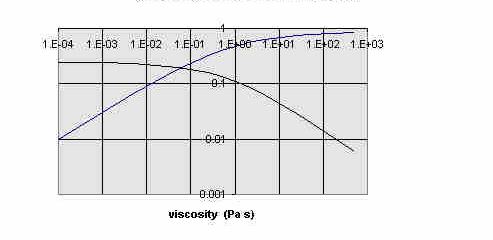
Figure 4. Phase and amplitude of liquid angular momentum vs viscosity.

It should be noted that an increase in amplitude of q_L (toward 1 as h® ¥ in Fig. 4) corresponds to a decrease in relative motion between can and liquid.

6.2  Period

The period variation was not compared directly with experiment for this study; however, the model does predict that it should increase by » 8 % as h increases from 10^-3 to 10³, as illustrated in Fig. 5.

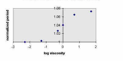
Figure 5. Variation of normalized model period with viscosity.

7  Comparison of Theory and Experiment

To compare theory with experiment, the value of eta in the model code was set at the viscosity appropriate to the liquid considered (value shown in Table I being h = 1, corresponding to glycerin). A record was then written to memory (every 10th point, separated in time by 0.05), which could be compared to the corresponding experimental record for that liquid. In all cases, the log decrement was computed by first finding the turning points in a given record. Then the peak-to-peak values were computed as previously indicated. Finally, an exponential fit to these peak-to-peak values was generated using Excel, from which the log half-decrement was obtained as the coefficient in the exponential fit. For the model sets, R²  =  1 in all cases as noted previously. The experimental data typically showed some amplitude dependence to the decay constant, but R² > 0.93 in all cases. The liquids which were considered in this study are indicated in Table II.

Table II. Liquids considered in the study.

Liquid        Viscosity (Pa·s)        Mass Density (g/cm³)
Acetone           3×10^-4                 0.79
Water                1×10^-3                1.00
Sugar water         7×10^-3                1.02
Vegetable oil       9×10^-2                0.86
Mineral oil         1×10^-1                0.82
Glycerin              1×10⁰                1.26
Corn syrup         3×10⁰                1.28
Honey                1×10¹                1.30
Corn starch         1×10³                1.03

The sugar water was made by dissolving 40% by weight of sucrose in water to produce a handbook listed viscosity of the indicated amount. All values of viscosity less than or equal to that of glycerin in Table II were obtained from handbooks. The value of h for liquids of higher viscosity was estimated relative to that of glycerin, using Stoke's Law. A small steel sphere was dropped in a test tube full of the liquid and the descent time was measured with a stopwatch. This time was then compared against the fall time using glycerin.

It should be noted that h is sensitive to temperature and therefore all experiments were performed at a laboratory temperature close to 23 C. In addition to the viscosities, the densities of the liquids are also provided in Table II. These were estimated from mass and volume measurements and their uncertainty is » 3%. For an ideal comparison of experiment and present theory, all liquids would have the same density, which is not possible. This complication will be discussed later. Theoretical damping (solid curve) is compared against experiment (data points with error bars in the log half-decrement) in Fig. 6.

Figure 6. Damping vs viscosity-Comparison of theory and experiment.

For this graph the single adjustable parameter of the model, c of Eq. (4) was set to 0.16-the value which was found by trial and error to give the best agreement with experiment. The (+/-) 16% 1s uncertainty (error bars of Fig. 6) is based on careful measurements done on glycerin, corn syrup, and the sugar water, using a set of 24 different records in each case. The range of the results for the three was from 14% to 17%, and smaller sample statistics with the other liquids suggested that an uncertainty of 16% is fairly representative of all cases. The uncertainty in h is much harder to quantify, particularly for the corn starch, which may be non-Newtonian. The estimate of its value at 1000 Pa·s could be wrong by as much as 50%. For the other liquids, the uncertainty in viscosity is probably in the neighborhood of 20%. In Fig. 6 two points are shown for water, to emphasize that there is amplitude dependence to the damping in this experiment. The larger value of the log half- decrement was obtained with the pendulum oscillating at a ten times larger amplitude. It was also noted that the R² declined from 0.99 for the least viscous liquids to 0.94 for the most viscous ones.

7.1  Influence of mass density differences

In the model, the mass of the pendulum has been assumed constant from one liquid to the next, which clearly is not true. The invariant quantity being the volume of the liquid, and since the can mass is only about one-tenth the liquid mass; we estimate from the densities of Table II that the mass of the acetone pendulum is » 80% that of water and that of the honey pendulum is » 130% that of water. These are the extremes of the variation for the liquids used in the present study. Future studies will consider whether the kinematic viscosity would be the better variable with which to make the comparison; i.e., division of h by the mass density. This seems reasonable since the damping constant, for a given viscosity, should decrease with increasing mass. Moreover, the kinematic viscosity is routinely used instead of absolute viscosity in engineering comparisons of gases. For the data of Fig. 6, the difference between the graph given and one based on kinematic viscosity is not great enough to warrant redrawing the figure. A significant reduction in the viscosity uncertainties, however, would make this meaningful.

8  Use of the can-pendulum as a viscosimeter

The reasonably good agreement between theory and experiment suggests that the system may be used as an instrument for measuring viscosity. Most liquids for which one would want to measure h are less viscous than glycerin. Therefore a power law fit to the low viscosity segment of Fig. 6 was performed. The resulting R² = 0.986 is not outstanding, but still close enough to unity that » 20% estimates in h should be possible from measured log decrements , by inverting the expression: log half-decr.  =  0.145h^0.3936, h < 1. Note that the log half-decrement has been used in these graphs, rather than the log decrement. To get the latter from the former, one need only multiply by a factor of 2.

9  Conclusions

It has been shown that some features of a liquid-filled can-pendulum can be readily understood, whereas others may be so complicated as to defy simple explanation. Pedagogically, it appears to be a system that is rich in new possibilities for improved teaching the old physics of classical mechanics. Particularly when the fluid of the can is inhomogeneous as by mixing solid particles with a pure liquid, unexpected behaviour can result. For example, it appears that dynamic organization of particles can then occur for some conditions, the nature of which are not yet understood. Planned future studies will attempt to understand these peculiar features. Future studies will also deal with the importance of pendulum mass, as well as size of the can. The theory which motivated the h^1/2 feature in Eqns. (4) and (5) also predicts that the dimensions of the can are important to the damping. Thus, an obvious follow-on experiment would be one to verify the functional dependence on can diameter.

References

[1]

R. D. Peters & Tim Pritchett, "The not-so-simple harmonic oscillator", Amer. J. Phys. 65, 1067-1073 (1997).

[2]

G. D. Nickas, "Reversing relative displacement in rolling fluids", Amer. J. Phys. 57, 907-912 (1989).

[3]

P. Bak, C. Tang, & K. Wiesenfeld, "Self-organized criticality", Phys. Rev. A ;98, 364- 374 (1988).

[4]

R. D. Peters, "Capacitive angle sensor with infinite range", Rev. Sci. Instrum. 64, 810-813 (1993). Note: For the present work a single unit with (+/-)  17.5^° range was used rather than the dual unit described in the reference, in which each unit was of range (+/-)  90^°. The electronics for this sensor may be purchased from TEL-Atomic Inc., Jackson, MI. Alternative electronics support is described on the WEBpage: http://physics.mercer.edu/peterpag/sens.htm.

[5]

H. P. Greenspan, The Theory of Rotating Fluids, p. 4, Cambridge Univ. Press London (1968).

[6]

A. Cromer, "Stable solutions using the Euler approximation", Amer. J. Phys. 49, 455-457 (1981).

[7]

An example is to be found in R. D. Peters, "Chaotic pendulum based on torsion and gravity in opposition" Amer. J. Phys. 63, 1128-1136 (1995).