TEL-Atomic Kater Pendulum Experiment
1 Objective
To measure the period of a physical pendulum of Kater type and from the data
estimate the acceleration of gravity, g, to a few parts in 10,000
in one laboratory period whose duration shall not exceed two hours.
2 Materials
1. TEL-Atomic Kater Pendulum,
the geometry of which is shown in Fig. 1; where the
hole nearest an end provides for rotation about axis-1, and
the other hole (approximately 2/3×37.4 cm from the
first is for axis-2).
Figure 1: Geometry of the TEL-Atomic Kater pendulum.
2. Slider
3. Timer accurate to 0.01%
4. Knife edge with clamp
5. Rigid vertical Post to support the clamped knife edge
6. Photogate
A photograph of the pendulum mounted to swing about axis-1 is provided
in Fig. 2. Similarly, Fig. 3 is a photograph corresponding to motion about
axis-2. Also shown and identified with labels in Figures 2 and 3
are various support items necessary to do the experiment, such as the Timer.
A variety of timers may be used, depending
on the mode of operation. For example, software of the KIS Interface
provides computer generated mean and standard deviation for a data set.
In choosing a timer, it is important to insure that it be
accurate (stable) to about 0.01%, which requires that the timer operate
with a quartz crystal oscillator.
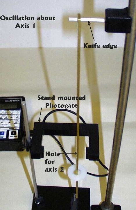
Figure 2: Pendulum mounted to swing about axis-1.

Figure 3: Pendulum mounted to swing about axis-2.
3 setup
3.1 Mounting the Pendulum
Mount the knife edge on the rigid vertical Post roughly 40 cm above the
surface of the table. Once mounted to swing about an axis,
the pendulum should execute motion in a plane that does not deviate
from vertical by more than a degree or two. If the knife edge is not level,
the pendulum may swing with a complex rocking motion
about an edge of the hole. Since this type of motion results in
very large errors, a leveling adjustment is necessary.
The adjustment is trivial when working with a Post that uses a
tripod base having three screws. If your Post is not of this type,
leveling can be accomplished by placing a small paper shim between
either the top edge of the clamp and the Post, or the bottom edge of
the clamp and the Post. It may be necessary to fold the paper
several times to obtain the necessary thickness.
Check for acceptability of the knife edge orientation as follows.
With a finger, initiate motion by displacing the
pendulum from equilibrium by an amount that is large compared
to the amount used for data collection (discussed later). When so doing,
purposely include a small out of plane component. If the resulting
out-of-plane rocking motion is fairly symmetric between right and left
turnings, and if this motion dampens quickly compared to the
desired planar motion; then the knife edge should be sufficiently level.
3.2 Positioning the Photogate
Position the photogate around the pendulum
as shown in Figures 2 and 3, with the pendulum hanging at rest in
equilibrium.
In relationship to the pendulum,
position the beam as shown in Fig. 4. Note that the beam
is located vertically at the midpoint of whichever hole is
not being used as an axis. The horizontal position is one for which
the beam is centered on the small segment of brass between one side of
the pendulum and the near edge of the hole.
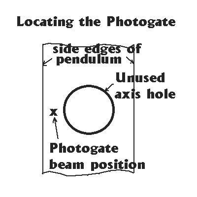
Figure 4: Positioning the photogate relative to the pendulum.
Once the photogate is properly aligned, no further adjustments are
necessary-except for slider positioning-
as the pendulum is swung first about one axis and then the other.
4 Procedure
4.1 Methodology
Either of two methods may be used to estimate g. Following the procedures
of this manual, both of them routinely yield an
estimate for g that is better than ten parts per ten-thousand.
In this manual, they are referred to as (i) the "quick" method and
(ii) the "preferred" method. If time permits, the latter technique is
recommended because it yields an uncertainty in g that is typically
about one-third that of the quick method.
The quick method uses the pendulum without a slider. Thus there is only
a single mass configuration of the instrument. In turn, there is a single
estimated period, T1 associated with axis-1 and likewise T2 for axis-2.
One must carefully estimate each of these periods by collecting enough
data to reduce the influence of random errors.
The preferred method collects a different T1 and T2 for each position
of the slider. If every possible position of the slider that does not
interfere with the photogate is investigated, then about 30 different data
sets result for each of T1 and T2 (total of 60 sets). Because a
regression analysis is performed with the mean of each set, fewer period
measurements per slider position are required, as compared to the
quick method. Although a full 60 data sets provide better appreciation
for the physics involved, the minimum number of slider positions necessary
for an accurate estimate of g can be as few as four or five. Thus the
total number of individual period measurements can be less than 200.
5 Data Collection
5.1 Mounting the Pendulum
When mounting the pendulum, be careful that the knife edge is
not offset laterally from
the center line of the pendulum by a great amount. Such an offset
causes the axis of rotation to move downward from its nominal
position, which is the top of the hole. To minimize this systematic
error, view the knife edge from the end as it is inserted through
the hole of the pendulum. Observing ambient light from the backside-
reposition, if necessary, for equality
on right and left sides of the knife edge. This process
works best by observing the hole area of the mounted pendulum
through a magnifying lens.
5.2 Initializing motion
Motion of the pendulum is initiated by simply pushing or pulling it with
a finger away from the equilibrium point, where the
photogate was aligned. The range of acceptable amplitudes of the
motion, during data collection, is somewhat narrow-approximately
0.25 cm to 1. cm peak to peak, at the position of the photogate.
For amplitudes less than » 0.25 cm, there is insufficient
motion for triggering.
Somewhere between 1 cm and 2 cm peak to peak motion, multiple
extraneous triggerings per cycle of the motion occurs. This is actually
useful, because it forces operation below the level at which amplitude
dependence on period is consequential. (For a zero to peak amplitude
of 40 mrad, the period is lengthened by
one part in ten-thousand. This amplitude of 40 mrad corresponds to
approximately twice the maximum amplitude permitted by the
triggering constraint.)
6 Quick Method Description
As noted above, the quick method uses the pendulum without the slider. About
each axis, collect approximately 100 period measurements. Do so with
two different mounting arrangements. In the first data
run, note which face of the pendulum is closest to the Post.
After 50 measurements are obtained, remove the pendulum from
the knife edge, then remount it with this face farthest from the Post;
i.e., rotate the pendulum 180 degrees about its length axis. In this
way, any significant systematic error associated with placement of
the pendulum on the knife edge may be discovered.
6.1 Calculations
Grouping all the T1 measurements together, and likewise for
T2, calculate the mean (designated by brackets) and standard
deviation for each period.
These calculations are made much simpler by means of the computer, or
a calculator with a statistics package.
6.1.1 Estimate of g
For a derivation of all equations which follow, refer to the Appendix.
To estimate the acceleration of gravity, use the formula (see Appendix
Eq. 8)
|
g = 4 p2 lm < T2 > / < T1 > 3 |
| (1) |
where lm = 0.24810 m is the spacing between the two axes.
6.1.2 Uncertainty in g
The uncertainty in g is obtained from the formula
|
Dg/g = [(Dlm/lm)2 + (2DT2/T2)2 + (3DT1/T1)2]1/2 |
| (2) |
The uncertainty in the axis separation distance
is Dlm » 0.00003 m; assuming that the
instrument has been manufactered according to specifications.
DT2 is the standard deviation of the T2 data set, and
similarly for T1. One can expect these to be in the neighborhood
of 3×10⁻⁴ s. Thus, Eq. 2 should yield a relative uncertainty in
g of the order of 1×10⁻³. Because of systematic errors,
it may be difficult to do substantially better than
one part per thousand by this method.
7 Preferred Method Description
Slider position is a variable which is indicated in the discussion
which follows.
The convention used is one for which zero corresponds to
the Slider being positioned at the end of the pendulum
farthest from axis-1. (One may want to refer to the picture
in Figure 3, which shows the Slider at the 7 cm position.)
If measurements over a large range of
slider positions are performed, a graph of the two periods
versus slider position should
look like that provided in Figure 5.
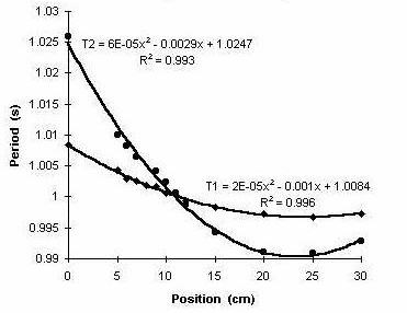
Figure 5: Variation of axis-1 and axis-2 Period over the full
range of Slider Positions.
Of course, such a wide range of slider positions is not necessary to
estimate g. As previously mentioned, only four or five positions are
really required. They must be chosen, however, to include the
position for which T1 = T2. One does not actually attempt to
place the slider at the exact position of equality; rather a graph
such as that of Figure 6 is produced.
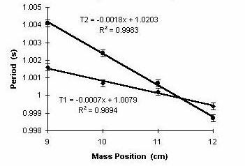
Figure 6: Period versus Slider position in the vicinity of period
matching.
Here, using Excel, a linear regression has
been separately performed on each of the T1 data and the T2 data.
Individual points correspond to the mean value of the period at a
given slider position.
From the regression analyses, the period T corresponding to
T1 = T2 = T is calculated (using the value of Slider position
which yields equality). Then the estimate for g, along
with its uncertainty is obtained from the following equations.
7.1 Calculations
7.1.1 Estimate of g
It is well known for the Kater pendulum that the system is equivalent
to a simple pendulum of length lm when the two periods are the
same. Since the period of a simple pendulum is well known to be
T = 2p[lm/g]1/2, we obtain by algebraic manipulation
the following simple expression
for our estimate of the acceleration of gravity:
with lm = 0.24810 m.
7.1.2 Uncertainty in g
The relative uncertainty in the g estimate is determined from:
|
Dg/g = [(Dlm/lm)2 + (2DT/T)2]1/2 |
| (4) |
Since the uncertainty in T is likely to be of the order of
3×10⁻⁴ s and Dlm/lm » 1.×10-4, this yields an expected uncertainty for
Dg/g » 6×10⁻⁴. Since the pendulum is also
mounted/dismounted a large number of times compared to the
quick method, this preferred method tends to "randomize"
some otherwise systematic errors. Thus the method is
typically two or three times more accurate than the
quick method.
File translated from TEX by TTH, version 1.95.
On 19 Oct 1999, 15:41.