Archer's Compound Bow-smart use of Nonlinearity
Randall D. Peters
Copyright, 2000, Randall D. Peters, Department of Physics
Department of Physics
1400 Coleman Ave.
Mercer University
Macon, Georgia 31207
Abstract
Using both theory and experiment, a compound bow has been studied, to assess
the benefit of its nonlinearity. Using a commercially available compound
bow, a measurement of force versus draw was performed. From this data, state
variables of the arrow during launch were theoretically estimated. The measured
launch speed of the arrow was found to be 13% smaller than the estimate,
and the difference is attributed to various forms of friction, which were
ignored. This study clearly demonstrates from physics principles the two
widely known and important advantages of the compound bow over earlier types-
improved precision and greater arrow launch speed.
1 Background
Adequate modelling of many physical systems has been long recognized by the
physics community as requiring modifications to linear theory. Historically,
the best known cases are ones which accommodated nonlinear correction via
perturbation analysis. Nevertheless, it was recognized that some phenomena,
such as thermal expansion, would not occur in the absence of nonlinearity.
Some historically important examples include the anharmonic potential
[1]-ultimately responsible for thermal expansion
and nonlinear acoustics [2], parametric phenomena
[3], subharmonic response in forced oscillations
[4], plasma waves and instabilities
[5], gravitational surface waves in water
[6], fluid drag
[7], and solitons
[8].
Because it is necessary, though not sufficient for chaos, nonlinear physics
has recently received great attention. Unlike earlier work, where nonlinear
terms resulted in small corrections to otherwise linear equations; nonlinearity
has in recent years become quintessential. Were it not for readily available
personal computers, this state would not have been attained so quickly, if
at all.
From the late 80's until the present, numerous nonlinear systems have been
examined, especially those that exhibit chaos. A resource paper concerned
with the subject is the one by Hilborn and Tufillaro
[9]. Among the cases cited there, it can be
seen that mechanical systems are especially popular among physics educators.
Of these mechanical systems, the pendulum has been a favorite; and several
commercial types are available for purchase
[10].
1.1 Evolution of a ``classic'' system
The archer's bow has been used for millenia. During its long history, there
was little substantive change to the physics of its operation, before the
patent awarded to H. Wilbur Allen in 1969 (U. S. Patent No. 3,486,495). As
compared to the ``compound bow'' invented by Allen, all early bow types could
be reasonably approximated by Hooke's law. For the compound bow, however,
restoring force and ``draw'' (string displacement from equilibrium) are far
from being proportional to one another.
2 Compound Bow Characteristics
For the bow tested (manufactured by Bear Archery, Gainsville, Florida) force
was measured with a large spring scale and draw was measured with a meterstick.
The results are shown in Figure 1, in which the breakover point (maximum)
in the vicinity of 0.2 m draw is quite pronounced.
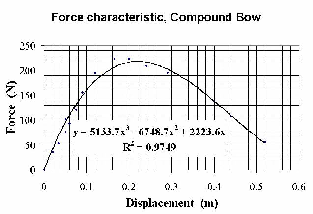
Figure 1: Force characteristic of the Compound Bow, Bear's "Realtree
Masterbucks".
The arrow-aiming position at full draw is seen to be only 52 N compared
to the maximum of about 220 N. Such a reduction, at four-fold, is large
compared to the majority of commercial bows.
The reduction in force for draw greater than 0.22 m results in two
significant benefits: (i) reduced stress on the archer while aiming, and
(ii) a smaller peak force of propulsion on the arrow without a loss in final
speed. Property (i) is evident from the graph; i.e., aiming is done where
the much reduced force to hold the arrow permits an improvement in precision.
The reason for benefit (ii) is not so obvious. In fact, it is a property
of the compound bow that was overlooked in an otherwise extensive treatment
of the physics of bow and arrow [11]. In Figure
8 of the appendix of Marlow's paper, though a force-draw curve for the compound
bow is presented; no use is made of the obvious difference between it and
the corresponding data of the recurve bow, also shown in the figure.
To compare the compound bow against other types, an idealized Hookeian (linear)
bow was selected according to the following criterion: the final speed of
the arrow launched by the two will be the same. In computing this final speed,
all friction will be ignored, including that of internal type due to anelasticity
associated with the bending of the (i) bow limbs, (ii) string, and (iii)
arrow. Additionally, the mass of the string and bow-limbs will be ignored,
which is a reasonable first order approximation (c.f. the paragraph immediately
above Fig. 8 in [11]).
With such approximations, theoretical estimates are straightforward and
demonstrate that the compound bow is dramatically superior to earlier bows,
such as the ``recurve''. Of course, this fact is already well known through
hands-on experience of those who have used both.
2.1 Integration Results
The force of Figure 1 was assumed to be fully applied to a target arrow of
length 0.81 m, diameter 0.89 cm, and mass
39.5 g. For purpose of integration, the data was approximated
by a cubic, the coefficients of which are indicated in Figure 1.
2.1.1 Acceleration
The resulting acceleration of the arrow as a function of time is shown in
Figure 2, where the top graph of the figure provides the force curve of the
Hookeian equivalent bow, mentioned above. As expected, the Hookeian acceleration
is seen to be one-fourth of a cosine curve.
Figure 2: Comparison of force (top) and arrow acceleration (bottom) for compound
and Hookeian bows.
The two bows show a profound difference in the history of arrow acceleration.
For the Hookeian bow, the acceleration is maximum at the time of arrow release,
whereas for the compound bow, the maximum occurs much later.
Using Newton's second law, a = F/m = dv/dt, the velocity
was obtained by numerically integrating
ňa·dt. Similarly, the arrow position
was obtained from ňv·dt. The results
are shown in the two graphs of Figure 3.
Figure 3: Comparison of arrow speeds (top) and position (bottom) for compound
and Hookeian bows.
3 Conclusions
The graphs of Figures 2 and 3 clearly show the benefit (ii) mentioned previously.
As can be seen from the top graph of Figure 3, the arrow leaves both the
compound bow and the Hookeian bow with the same speed (maxima of the graphs).
As seen from the Figure 2 lower graph, however, the peak acceleration of
the arrow is dramatically smaller for the compound
bow-5500 m/s2 compared to 7600 m/s2. This
acceleration derives from the bow force acting at the back of the arrow,
which because of inertia results in a tendency for the arrow to ``buckle''.
The figure therefore shows that a smaller diameter arrow may be safely and
accurately used with the compound bow. An added benefit is that a smaller
mass arrow may be used, resulting in a higher launch speed.
4 Goodness of Model
To test the theory presented above, arrow launch speed was measured by shooting
an arrow horizontally and measuring its drop through a known distance. Shooting
at a target 26 m away, the drop was measured to be 1.1 m, from
which the launch speed was calculated to be 55 m/s. This being 13% smaller
than the peak value of Figure 3, the difference is reasonably attributed
to friction losses of the type mentioned earlier. It thus appears that the
approximations previously mentioned are reasonable ones for a first order
model.
5 Conclusions
The compound bow is an example of a device which uses nonlinearity to great
advantage. Like musical instruments, it has evolved through trial and error;
and it appears that very little theoretical physics was used in the process.
Nevertheless, the present paper shows that the compound bow is amenable to
at least partial, yet meaningful theoretical treatment. More refined analysis
could even allow for better archery designs. Regardless, the approximations
of the present treatment appear useful- at least for gaining conceptual insights
into the physics of nonlinearity.
6 Acknowledgement
Assistance in this effort, provided by Dr. Douglas T. Young, is much appreciated.
7 APPENDIX-Basis for ``Breakover''
The physics responsible for the breakover in the compound bow is fundamentally
simple. The string passes around a pair of elements, on the ends of each
limb, that are either (i) an eccentric, or (ii) a cam. Although quantitative
differences result depending on the choice of one or the other, their qualitative
properties are similar. The shape of a cam deviates from the simple circle
of an eccentric. Careful design of this shape permits a small ratio of aim-force
to max-force. For example, in the presently described bow, the ratio is about
one-fourth. When using an eccentric, the ratio is larger, usually not less
than one-half.
The specific free-body treatment of the forces and torques present in a drawn
compound bow is prohibitively complicated. For present purposes, there is
little merit to such an analysis, since we are seeking conceptual understanding.
To assist this understanding, consider the eccentric of Figure 4.
Figure 4: Coordinate system for analyzing the properties of an eccentric.
Shown is a pulley of radius R in which the center is offset by an amount
r from the axis of rotation, which is located at the origin of coordinates.
The pulley experiences linear torsional restoration about the axis, and a
force of constant direction is applied at the contact point P through
the inextensible rope which wraps around and is secured at the other end
to the eccentric. Note that a change in q requires
that xF must also change, except when r = 0. It is
this change that is responsible for the ``breakover'' characteristics, due
to the variation in moment arm distance with angle. In particular, the ratio
r/R is important in this regard.
7.1 Theoretical Analysis
For purpose of analysis, an x-y Cartesian coordinate system was selected.
A line connecting the origin and the center of the pulley is horizontal when
q = 0 , corresponding to
the reference position. The reference position results when (i) F
has been set to zero, and (ii) the pulley mass and rope mass are assumed
negligible.
For r = 0 , the idealized system obeys Hooke's law (linear,
subscript L ); so that the restoring force is proportional to the torsion
constant, kL , as follows.
For nonzero r , the resulting nonlinear system obeys the following
equations:
and
Eqns. (2) and (3) are obtained by recognizing that (i) the moment arm of
the force is xF =
R - r cos q and
(ii) the vertical position yF does not equal
R q except when the offset is zero; i.e.,
it is less by the vertical travel of the cord contact point, P, given by
r sin q.
Breakover does not occur unless r/R exceeds a critical value, and later analysis
will show this to be rc/R = 0.637. It is interesting
to compare force versus draw in the vicinity of rc, as shown in
Figure 5. In addition to the case for which r = rc,
a curve is shown in which the ratio is 40% smaller than critical and another
in which it is 40% larger. The circle for a given case indicates the value
of yF for which q =
p/2.
Figure 5: Force vs draw around critical offset.
7.1.1 Comparison of Theory and Experiment
for an Eccentric
An eccentric was constructed to test the equations provided. Having a radius
of R = 12.5 cm and offset of r =
6.2 cm, it was operated with the axis of rotation vertical to
eliminate the influence of its mass. The torsion constant
kL » 2000 g/rad
of Eq.(1) resulted from a coiled spring (750 g/cm) acting 2.6 cm
from the axis (by means of a pulley). The force versus displacement was measured
with a spring scale and a meterstick. Comparison of theory and experiment
for this case, in which r/R = 0.5 is shown in Figure 6, where
theory is the solid line.
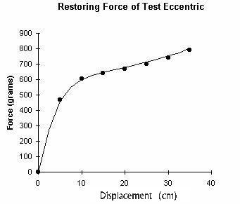
Figure 6: Comparison of theory and experiment with a test eccentric.
7.2 A ``cardinal'' point
From Eqns. (2) and (3), the derivative of force with respect to position
is given by
|
dF
dy
|
= |
dF
dq
|
/ |
dy
dq
|
= |
k [(R - r cos q) - r q sin q]
(R - r cos q)3
|
|
|
(4) |
from which an interesting ``operating'' point is found to be
q =
p/2 . Here, the derivative assumes the
simple form
Using these expressions, a compound vertical seismometer was built, in which
Eq. (5) provides the force ``constant" with which a mass oscillates vertically.
In this case, the weight of the mass provides a constant force equal in magnitude
to the restoring force of the eccentric at the operating point. It was the
similarity of this (unpublished) seismometer and the compound bow which motivated
the present study. It is instructive to compare Eqns. (4) and (5) to the
equivalent Eq. (1) when r = 0 .
7.2.1 Potential Energy
The potential energy as a function of position relative to the cardinal point
was obtained by stepping through closely spaced values of
q to produce associated sets of F
and y . The potential energy was then obtained from a simple numerical
approximation to - ňF(y)dy. The
figures which follow were produced using QuickBasic and PSET. A ``screendump"
algorithm was used to transfer the monitor displayed graphs into memory.
For zero offset, the well known Hooke's law case results. As the offset is
increased from zero, anharmonicity is introduced, as shown in Figure 7.
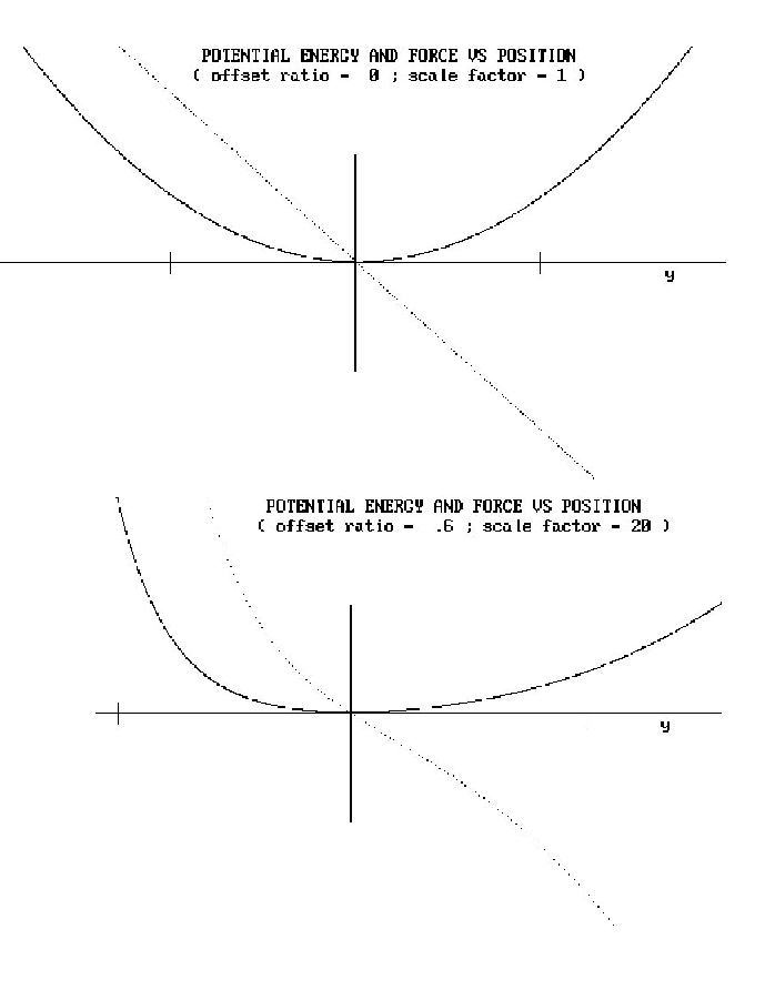
Figure 7: Introduction of nonlinearity through offset.
Here, and in all cases which follow, the fainter curve is the force, and
the darker curve is the potential energy. In addition to the vertical axis
at y = 0 , the graphs in some cases show vertical
``tick" marks corresponding to q =
p/4 and
3p/4 .
With non-zero r , the force ``constant" becomes a function of
y . For the p/2 operating point,
this ``constant" can be made to vanish according to the following condition,
using Eq.(5)
|
dF
dy
|
=
0 , r = |
2
p
|
R = 0.637 R =
rc |
|
(6) |
Thus, a region can exist for which the period of oscillation may be large.
It is enlightening to consider a graph of energy/force both at the critical
value r = rc and slightly above it, as
shown in Figure 8.
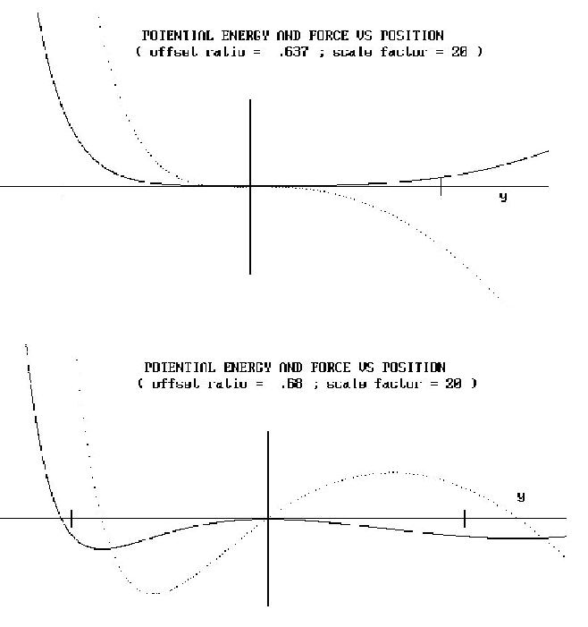
Figure 8: Conversion to a double-well potential as r
> rc.
Observe that the ordinate scale for all the nonlinear cases has been expanded
by a factor of 20, as compared to the Hookeian case. This reflects the increased
sensitivity of the instrument as
r ® rc . In all cases
the axes are linear, and the vertical axis (located at y = 0) corresponds
to q =
p/2 .
It is seen that the potential is generally anharmonic, so that the magnitude
of the restoring force is greater for upward ( y
< 0 ) as compared to downward
( y > 0 ) displacements.
For large external excitation, this would result in harmonic distortion.
When r = rc, there exists a ``flat" region in
the potential well, as shown in Fig. 8. This ``deadband" region might be
useful for some sensing applications.
Notice that when r >
rc, a double-well potential results, in which there
are three equilibrium points. The one at y = 0 is
unstable; and there are two stable equilibrium points on either side of zero.
Apart from the asymmetry, this bistable system should in some ways be similar
to the Duffing oscillator.
References
-
[1]
-
W. C. DeMarcus, ``Classical motion of a Morse oscillator,'' Am. J. Phys.
Vol. 46 (7), 733-734 (1978).
-
[2]
-
R. T. Beyer, ``Nonlinear acoustics,'' Am. J. Phys. Vol. 41 (9), 1060-1067
(1973).
-
[3]
-
L. Adler and M. A. Breazeale, ``Parametric phenomena in physics,'' Am. J.
Phys. Vol. 39 (12), 1522-1527 (1971).
-
[4]
-
A. Prosperetti, ``Subharmonics and ultraharmonics in the forced oscillations
of weakly nonlinear systems,'' Am. J. Phys., Vol. 44 (6), 548-554 (1976).
-
[5]
-
C. L. Grabbe, ``Resource letter: PWI-1 Plasma waves and instabilities,''
Am. J. Phys., Vol. 52 (11), 970-981 (1984).
-
[6]
-
J. Wu and I. Rudnick, ``An upper division student laboratory experiment which
measures the velocity dispersion and nonlinear properties of gravitational
surface waves in water,'' Am. J. Phys. Vol. 52 (11), 1008-1010 (1984).
-
[7]
-
V. K. Gupta, G. Shanker, and N. K. Sharma, ``Experiment on fluid drag and
viscosity with an oscillating sphere,'' Am. J. Phys. Vol. 54 (7) 619-622
(1986).
-
[8]
-
P. J. Hansen, and D. R. Nicholson, ``Simple soliton solutions,'' Am. J. Phys.
Vol. 48 (6), 478-480 (1980).
-
[9]
-
R. C. Hilborn and N. B. tufillaro, ``Resource Letter: ND-1: Nonlinear dynamics,''
Am. J. Phys. Vol. 65 (9), 822-834 (1997).
-
[10]
-
J. A. blackburn and G. L. Baker, ``A comparison of commercial chaotic
pendulums'', Am. J. Phys. Vol. 66 (9), 821 -830 (1998).
-
[11]
-
W. C. Marlow, ``Bow and arrow dynamics'', Am. J. Phys. 49 (4), 320-333 (1980).
Return to Homepage
File translated from TEX by
TTH,
version 1.95.
On 9 Jun 1999, 10:39.