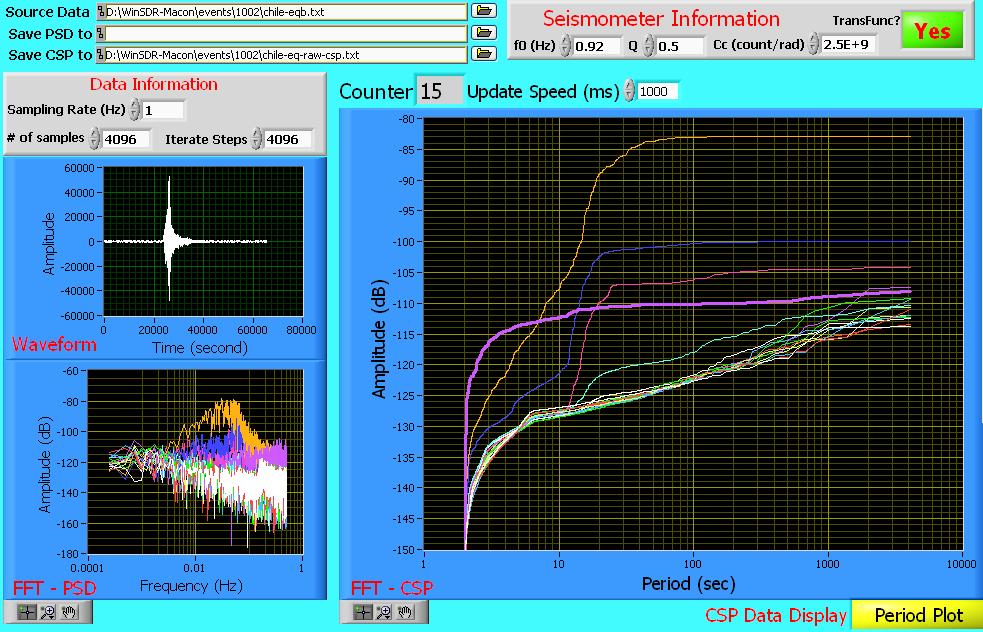
Figure 1. Graphical composite showing (i) a time record (upper left), (ii) its associated set of PSD's (lower left), and (iii) the CSP set obtained from the PSD set by integration (large graph).
Randall D. Peters
Physics Department, Mercer University
Macon, Georgia
Copyright August 2010
Abstract
Because of inherent nonlinearities, low frequency eigenmode oscillations are expected to modulate higher frequency motions of the Earth. Such amplitude modulation is expected to be visible during large earthquakes, which are known to excite free (eigenmode) oscillations of the Earth. A means for observing the modulation, as illustrated in the materials that follow, is to perform frequency domain calculations on the 'rectified' signal, as opposed to the customary calculations that are performed on the 'raw' signal.
Software Tools
Evolution of the spectral content of a signal is easier to analyze in a cumulative spectrum than in a (traditional) density spectrum. Obtained by integrating over frequency (or period) of the power spectral density (PSD), the cumulative spectral power (CSP) is much less cluttered [1]. Thus a set of time-differing (sequenced) CSP plots can be overlaid in a single graph as shown in Fig. 1.
Figure 1. Graphical composite showing (i) a time record (upper left),
(ii) its associated set of PSD's (lower left), and (iii) the CSP set
obtained from the PSD set by integration (large graph).
The time signal was recorded by a Macon, Georgia VolksMeter [2] located in the Seismic Lab of the Physics Department of Mercer University. Though the earthquake displayed in the figure (large Chile event of February 2010) was archived at a sample rate of 10 per s, only 10% of the data (1 Hz) was used in generating all the graphs of the present article.
Each of the frequency-domain graphs (PSD and CSP) comprises 16 overlaid plots. Each plot was obtained from a record piece having a duration of 4096 s. The 16 contiguous pieces were sequenced to cover the total record from start to finish.
The reduced-clutter nature of the CSP compared to the PSD is immediately evident from Fig. 1, by comparing the largest graph to the lower left graph. The abscissa is different for the two cases; i.e., PSD's are plotted versus frequency, whereas the CSP's are plotted versus period. For this log-log PSD case, if it were instead plotted vs period; a mirror image of the graph shown would result.
For Fig. 1, a given PSD was obtained by operating on the `raw' signal with the Cooley-Tukey FFT algorithm. The associated CSP was then obtained from the PSD by integration. Before showing similar graphs, but those obtained by operating on the `rectified' signal-a discussion of amplitude modulation is first now provided.
Figure 2. Simulations of (i) the time domain (upper left) of an
amplitude modulated signal, (ii) the spectrum of the raw signal
(upper right),
and (iii) the spectrum of the rectified signal (bottom).
The graphs of Fig. 2 were generated using Excel. The equation describing the time graph is
| (1) |
where A = 1 , M = 0.5 , wc = 6.2832 × 0.25 s-1 , and wm = 6.2832 × 0.002 s-1
Observe the striking difference between the two spectra shown in Fig. 2. These were obtained by using the Fourier analysis (FFT) tool of Excel. One could use a trigonometric identity to operate on Eq. (1) and obtain the sum/difference frequency terms that would show up as sidebands to the 0.25 Hz spectral line in the raw spectrum, only if a narrow spectral region were being viewed. They are not visible in the full-width spectrum that is here displayed by means of the log-abscissa.
From its time domain appearance, many are probably surprised by the fact that the spectrum of the raw signal (as presented and which is typical) appears to provide no information concerning the modulation signal which has a frequency of 0.002 Hz. On the other hand, this 2 mHz `information' component is unmistakeable in the spectrum of the rectified signal. For this case, and also for the other cases of this paper, rectification involves what is called `half-wave' in radio terminology. In other words, all negative-going parts of the signal are `clipped-off'. One could also use the absolute value of signal components to accomplish `full-wave' rectification.
One `artifact' of the rectification process is visible in the bottom graph of Fig. 2-the introduction of a 2nd harmonic component of the `carrier'. In other words, in addition to the spectral line at 0.25 Hz corresponding to the carrier, there is also the spurious line having the frequency of 0.5 Hz. Only half of this line is visible, because the Nyquist (cutoff) frequency for the data was 0.5 Hz.
On the basis of Fig. 2, it is reasonable to expect that a low frequency component of earth motion might, for reason of amplitude modulation, be invisible in a conventional PSD. It is thus worth-while to compare two spectra-one being conventional and the other using the rectified signal. That the two can be significantly different in meaningful ways is illustrated by comparing the graphics of the next Fig. 3 with those of Fig. 1.
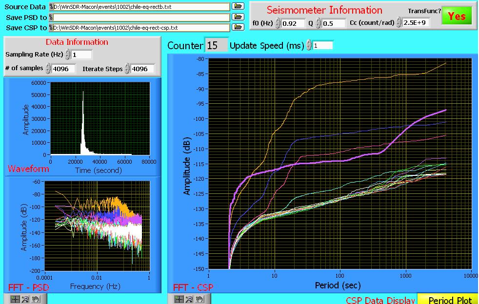
Figure 3. Analgous to Fig. 1 but using the rectified signal
rather than raw signal.
The most striking difference between Figures 1 and 3 is seen in the 6th plot of total 16, that has been highlighted by the thicker line in the CSP graph of each figure. Corresponding to the time interval from 20,480 s to 24,576 s, this 6th segment is seen from the time graph to coincide with highly energetic parts of the earthquake record. Notice the slope change that occurs at about 400 s period in the rectified signal CSP no. 6 (highlighted) plot. This change is not present in Fig. 1, and and so the increase in total power for periods longer than 400 s implies amplitude modulation.
It is significant that the major difference occurs only for periods greater than 400 s, corresponding to 2.5 mHz. This is roughly the transition frequency that separates free-oscillations from other seismic motion types.
Another graphical tool employed for this study involved replotting CSP values as a function of time, for select values that are a small subset of the 2048 frequencies used in figures 1 and 3. These are shown in figures 4 and 5.

Figure 4. Time dependence of the cumulative spectral power
for select (octave separated) frequencies. Calculations
used the raw signal.
Figure 5. Analagous to Fig. 4, except calculations used
the rectified signal.
Differences in the `variations around the peak' of figures 4 and 5 again suggest that eigenmode oscillations served to amplitude modulate higher frequency seismic motions when our planet was most energetic because of the earthquake. Nonlinearity that produces harmonnics (or modulation in the present case) has been sufficiently studied [3] to expect that its influence should be proportional to the square of the power of the responsible vibrations. The modulation is thus expected to be visible (as noted) around the time of the earthquake peak.
Conclusion-Mechanical Systems in General
Nonlinearity is pervasive in nature and too many scientific endeavors have tried to ignore it. This has been especially true of most treatments of energy dissipation in mechanical oscillators. A paper that discusses the matter in detail involves pendulum damping [4]. The following, important and very real possibility is thus virtually unknown:
Because of nonlinearity, not all the modes of vibration of a mechanical system reveal themselves through traditional frequency domain analysis methods. Low frequency oscillations may be hidden by way of their amplitude modulation of higher frequency modes. A simple means for testing whether this is the case is to do spectral calculations on the rectified, rather than the raw signal.
The first occasion for the author to discover this phenomenon was in his studies of seismocardiography. These grew out of his idea to use a geophone to study the heart [5]. When the heart beats, it excites a variety of chest-wall modes that typically peak around 10 Hz. Heart and respiration rates of the subject are frequently very visible in the time records. Nevertheless, the same features may not be at-all obvious in the associated frequency-domain records. Similar results were discovered in the analyzis of some electrocardiograms. In all cases, as with the present treatment of seismic data involving an earthquake-the low frequency modes that have been hidden because of amplitude modulation effects-become visible in the frequency domain graphs when the FFT is applied to the rectified signal rather than to the raw signal.
Bibliography
[1] Peters, Randall D., ``A new tool for seismology, the Cumulative
Spectral Power" (2007), online at
http://arxiv.org/ftp/arxiv/papers/0705/0705.1100.pdf
A related paper by Lee, S.C & Peters is
``A new look at
an Old Tool-the Cumulative
Spectral Power of Fast-Fourier Transform Analysis",
online at http://arxiv.org/ftp/arxiv/papers/0901/0901.3708.pdf
[2] Peters, Randall D., "State of the Art Digital Seismograph" (2006),
online at http://psn.quake.net/Volksmeter/State-of-the-art_Digital_Seismograph.pdf
[3] Peters, Randall D. "Temperature Dependence of the
Nonlinearity parameters of Copper", PhD dissertation, The University
of Tennessee (1968).
[4] Peters, Randall D., ``Nonlinear damping of
the linear pendulum'' (2003),
online at http://arxiv.org/pdf/physics/0306081
[5] Shell, Jared et al, ``Three-axis seismocardiography using a low-cost
geophone accelerometer'' (2007), abstract online at
http://www.fasebj.org/cgi/content/meeting_abstract/21/6/A1261-c